A convex optimization problem is a problem where all of the constraints are convex functions, and the objective is a convex function if minimizing, or a concave function if maximizing.
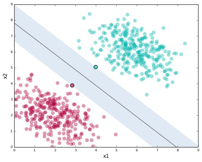
On the linear classifier on the SVM which we told here Linear Support Vector Machine, The linear classifiers can be an effective tool in the big data, the most important linear classifier is SVM (Support Vector Machine).
The idea of SVM is take all of the possible hyperplane that can seperate the data which the largest margin.
Convex Optimization Problem
The convex sets \(X ⊂ ℝ^d\) is a set if only if the line segment connecting any two point in X entire lies within in X. For example a convex sets if we have two points and we draw line between two points, and all of the line lie on the set X no mater you choose which any points. Mathematically we can describe as
\[\forall x_1, x_2 \in X, \ \forall \theta \in [0,1] : (1- \theta) x_1 + \theta x_2 \in X\]Convex Functions is a function \(f : ℝ^d \rightarrow ℝ\) is convex if and only is the set above the graph is convex, that is,
\[\forall x_1, x_2 \in ℝ^d, \ \forall \theta \in [0,1] : f((1- \theta) x_1 + \theta x_2)) \leq (1 - \theta) f(x_1)+ \theta f(x_2)\]\(f((1- \theta) x_1 + \theta x_2))\) is a line function which connecting from point one and point two. So the convex line function must be less or equal to the line that is drawed between one point to the other point \((1 - \theta) f(x_1)+ \theta f(x_2)\).
Concave
A function f is concave if and only if the -f is convex
How can I check that f is convex?
We can check the covexivity by using the theorem second-order condition. f is convex if and only if the hessian matrix H(x), which generated by using second derivatif of the function, is positive semi-definite for all \(X \in ℝ^d\)
To check whether function is convex we try on for example function which map from \(ℝ \rightarrow ℝ\)
\[f(x) = 2x - 3x^2 + 7\] \[f'(x) = 2 - 6x\] \[f''(x) = - 6 < 0\]So the f function is not convex. However, if we put minus on the function we can get that f is concave as shown below
\[f(x) = -(2x - 3x^2 + 7)\] \[f'(x) = -(2 - 6x)\] \[f''(x) = 6 > 0\]Another example is when we try on the high dimentional dor example mapping from \(ℝ^2 \rightarrow ℝ\)
\[f(x,y) = x^2 + y^2\] \[\nabla f(x,y) = \begin{pmatrix} 2x\\ 2y \end{pmatrix}\] \[H_f (x,y) = \begin{pmatrix} 2 && 0\\ 0 && 2 \end{pmatrix}\]You can see that positive semi definite matrix from hessian, you can also calculate the determinant of the hessian \(det(H_f (x,y)) = 4\) which is greater than zero.
The determinant of a Hessian matrix can be used as a generalisation of the second derivative test for single-variable functions. If the determinant of the Hessian positive, it will be an extreme value (minimum if the matrix is positive definite). If it is negative, there will be a saddle point. If it is 0, another test must be used.
Convex Optimization Problem
The definition of an optimization problem (OP) is the problem of minimizing convex functions over convex sets.
Then, we want to apply, is the SVM is a convex OP?
\[\underset{\gamma, b \in ℝ, w \in ℝ^d, \xi_i,...\xi_n \geq 0 }{\max} \gamma \ \ \ \ s.t. \ \ \ \ y_i \ ( w^T x + b ) \geq \| w \| \ \gamma , \ \ \forall i = 1,...,n\]However, the standard form of an optimization problem is minimize not maximize, so we need to update this SVM into Convex Optimization Problem.
SVM is a Convex Optimization Problem
We rewrite the SVM so it match with the convex form
\[\underset{ b \in ℝ, w \in ℝ^d }{\min} \frac{1}{2} \| w \|^2 \ \ \ \ s.t. \ \ \ \ 1 - y_i \ ( w^T x + b ) \leq 0 \ \ \forall i = 1,...,n\]The basic idea of the proof is that the SVM results in a linear classifier \(f(x) = sign(w^T x + b)\), the parameters (w,b) of which are not unique.
Idea is if it helps, we could restrict in the SVM OP our search for w to ws that have some nice norm, and we would still search the space of all linear classifiers. For reasons that will become clear below, we choose the restriction \(\| w \| = \frac{1}{\gamma}\), by setting \(\lambda := \frac{1}{ \| w \| \gamma }\)
Proof:
\[\underset{\gamma, b \in ℝ, w \in ℝ^d }{\max} \gamma \ \ \ \ s.t. \ \ \ \ y_i \ ( w^T x + b ) \geq \| w \| \ \gamma , \ \ \forall i = 1,...,n\] \[\underset{\gamma > 0, b \in ℝ, w \in ℝ^d }{\min} \frac{1}{\gamma} \ \ \ \ s.t. \ \ \ \ y_i \ ( w^T x + b ) \geq \| w \| \ \gamma , \ \ \forall i = 1,...,n\] \[\underset{\gamma > 0, \lambda > 0, b \in ℝ, w \in ℝ^d }{\min} \frac{1}{ 2 \gamma^2} \ \ \ \ s.t. \ \ \ \ y_i \ ( \lambda w^T x + \lambda b ) \geq \lambda \| w \| \ \gamma , \ \ \forall i = 1,...,n\] \[\underset{\gamma > 0, \lambda > 0, \bar{b} \in ℝ, w \in ℝ^d }{\min} \frac{1}{ 2 \gamma^2} \ \ \ \ s.t. \ \ \ \ y_i \ ( \lambda w^T x + \bar{b} ) \geq \lambda \| w \| \ \gamma , \ \ \forall i = 1,...,n\] \[\underset{\gamma > 0, \lambda > 0, \bar{b} \in ℝ, w \in ℝ^d }{\min} \frac{1}{ 2 \gamma^2} \ \ \ \ s.t. \ \ \ \ y_i \ ( \frac{w^T}{ \| w \| \gamma} x + \bar{b} ) \geq 1 , \ \ \forall i = 1,...,n\] \[\| \bar{w} \| = \| \frac{w}{ \| w \| \gamma } \| = \frac{1}{\gamma}\] \[\underset{\gamma > 0, \lambda > 0, \bar{b} \in ℝ, \bar{w} \in ℝ^d }{\min} \frac{1}{2} \| \bar{w} \|^2 \ \ \ \ s.t. \ \ \ \ y_i \ ( \bar{w}^T x + \bar{b} ) \geq 1 , \ \ \forall i = 1,...,n\]On the similar way, we can formulate a soft-margin SVM as convex optimization problem. Linear soft-margin SVM in convex form.
\[\underset{b \in ℝ, w \in ℝ^d, \xi \in ℝ^n }{min} \ \ \ \frac{1}{2} \| w \|^2 + C \sum_{i=1}^{n} \xi_i\] \[s.t. \ \ \ \ 1 - \xi_i - y_i ( w^T x_i + b ) \leq 0 , \ \ \ - \xi_i \leq 0 \ \ \forall i = 1,...,n\]What is the core idea to transform the SVM into the form of a convex optimization problem?
The parameter (w,b) of a linear classifier \(f(x) = w^T x + b\) are unique only up to multiplication by positive scalar. Therefore we can rescale the parameter w in the problematic (non-convex) term ‖ w ‖ occuring in the SVM.
How to Solve Convex OPs and SVM
Convex OPs is easy to solve. why are convex OPs easy to solve? Because for convex problem every locally optimal point of a convex optimization problem is also globally optimal.
Gradient Descent
Gradient descent is an optimization algorithm used to minimize some function by iteratively moving in the direction of steepest descent as defined by the negative of the gradient.
For unconstrained problems, we can iteratively move into direction of steepest decent (negative gradient direction) of the objective function.
initialize x0
for t = 1 : T do
  xt+1 := xt - λt ∇ f0(xt)
endfor
λt is called step size or learning rate.
With a high learning rate we can cover more ground each step, but we risk overshooting the lowest point since the slope of the hill is constantly changing. With a very low learning rate, we can confidently move in the direction of the negative gradient since we are recalculating it so frequently. A low learning rate is more precise, but calculating the gradient is time-consuming, so it will take us a very long time to get to the bottom.
A typical choice: \(\lambda_t = \frac{1}{t}\). it is the safe for learning rate, but people usually try another learning rate.
Applying Gradient Descent to SVM OP
\[\underset{b \in ℝ, w \in ℝ^d, \xi \in ℝ^n }{min} \ \ \ \frac{1}{2} \| w \|^2 + C \sum_{i=1}^{n} \xi_i\] \[s.t. \ \ \ \ 1 - \xi_i - y_i ( w^T x_i + b ) \leq 0 , \ \ \ - \xi_i \leq 0 \ \ \forall i = 1,...,n\]If we apply gradient descent to SVM what could be the problem? The problem is the constraints.
The linear SVM can be equivalently re-written as follows (unconstrained linear soft-margin SVM):
\[\underset{b \in ℝ, w \in ℝ^d }{min} \ \ \ \frac{1}{2} \| w \|^2 + C \sum_{i=1}^{n} max (0, 1 - y_i ( w^T x_i + b ) )\]we can get the form like that because,
\[1 - \xi_i - y_i ( w^T x_i + b ) \leq 0 , \ \ \ - \xi_i \leq 0\] \[\xi_i \geq 1 - y_i ( w^T x_i + b ) , \ \ \ \xi_i \geq 0\] \[\xi_i \geq max (0, 1 - y_i ( w^T x_i + b ) )\]Subgradient Descent
The another problem is f0 is not differentiable, In this case we consider the subgradient descent which is the gradient descent but using the subgradient in place of gradient.
\[\sum_{i=1}^{n} \nabla max (0, 1 - y_i ( w^T x_i + b ) ) = \begin{cases} \sum_{i=1}^{n} \nabla (1 - y_i ( w^T x_i + b )),& \text{if } y_i ( w^T x_i + b ) < 1 \\ 0, & \text{otherwise} \end{cases}\]Logistic Regression
The second option is replace ‘hinge’ function. Logistic Regression is diferentiable, so we can solve it using gradient descent.
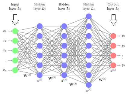
Logistic regression is a classification algorithm used to assign observations to a discrete set of classes. Unlike linear regression which outputs continuous number values, logistic regression transforms its output using the logistic sigmoid function to return a probability value which can then be mapped to two or more discrete classes.
By rewritting the function and using the Logistic Regression,
\[\underset{b \in ℝ, w \in ℝ^d }{min} \ \ \ \frac{1}{2} \| w \|^2 + C \sum_{i=1}^{n} ln (1 + exp(- y_i ( w^T x_i + b ) ))\]But the gradient descent, subgradient descent and logistic regression is too slow. Because we sum of all of the data points \(\sum_{i=1}^{n}\). So it will costly on the big data.
But, we don’t need to evaluate of full loop. We just imagine all data points were the same or duplicated. So all my data is just a big point, in this case all of our data is just factor of n.
\[\sum_{i=1}^{n} max (0, 1 - y_i ( w^T x_i + b ) ) = n \cdot max (0, 1 - y_i ( w^T x_i + b ) )\]Real data is usually less extreme which is not exact duplicates, but yet contains lots of redudancy. Unnecessary to evaluate the full subgradient in every iteration.
So to handle this there is algorithm that called Stochastic Gradient Descent (SGD) which run much faster runing based on this idea.
Stochastic Gradient Descent (SGD)
Stochastic gradient descent is an iterative method for optimizing an objective function with suitable smoothness properties. It can be regarded as a stochastic approximation of gradient descent optimization, since it replaces the actual gradient by an estimate
initialize (b,w)_0
for t = 1 : T do
    // Randomly select B many data points
    // denote their indexes by I ⊂ {1,...,n}(i.e. |I| = B)
    // update (b,w)_t+1 := ....
    // it's same as gradient descent but we apply just only B many point in the sum.

endfor
B is the Batch size which needs to be choosen a priori.
What is the different between Gradient Descent and Stochastic Gradient Descent?
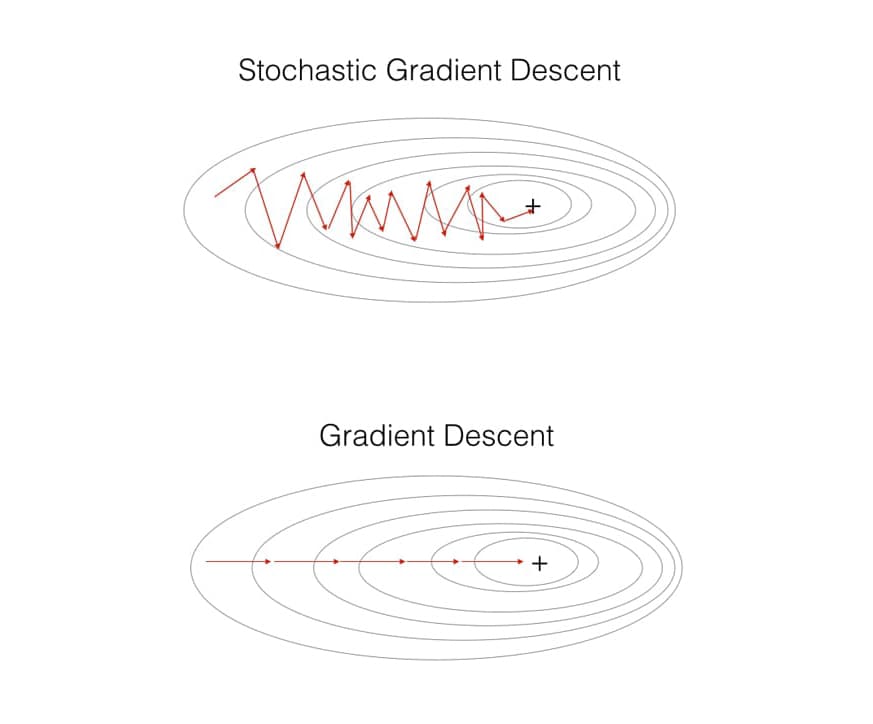
The practical point of view, you can see that the Gradient Descent move perfectly to the minimum point. However the Stochastic Gradient Descent will look like a zigzag, it is because we just calculate the subset of the data.
Is it guaranted to work?
There is a theory on SGD convergences. Consider Stochastic Gradient Descent using the learning rate λt = 1/t. Then, under mild assumptions, SGD converges with high probability to a stationery point with rate
\[f_0 (x_t) - f_0 (x_{local}^*) \leq O( \frac{1}{t})\]Remark that this holds also for non-convex function.
Software
An extremely fast implementation of SGD applied to the linear (soft-margin) SVM and logistic regression is contained in Vowpal Wabbit which is the industry standard in ad prediction.
The discussion is VW trades speed for accuracy, so use it only when really necessary for example in big data. Otherwise use LIBLINEAR, a more accurate and still relatively fast solver SVM and LR.
Conclusion
- Convex Optimization Problem (OP), optimize convex function over convex set.
- Why convexity? cannot get stuck in local optimum
- SVM can be formulated as convex OP,
- unconstrained formulation of SVM
- gradient descent slow for SVM
- solution: Stochastic Gradient Descent

 Linear Support Vector Machine