Linear Support Vector Machine

Support Vector Machine (SVM) is a machine learning algorithm which can be used for both regression or classification problem.

It is an supervised algorithm in Machine Learning and mostly used in classification problems. Machine Learning is about computer learning from data how to make accurate predictions.

Formal problem setting and terminology, for example we are given the training data which usually denote as input x₁,…,x_n and label y₁,…,y_n. The aim is to compute a function f (called classifier or predictor) which predicting the unknown label y of a new input x . For example in k-nearest neighbor algoritm.

In SVM we plot data points as points in an n-dimentional space (n being the number of feature that you have). The value of the feature be in the particular coordinate.

Linear Classifiers

Math Notation

The math notation for Machine Learning is very standard. we will give list the notation below

• Vectors v ∈ ℝ^d are thought of as column vectors and denoted with boldface lettters.
• Scalars s ∈ ℝ are denoted with normal letters
• Matrices M ∈ ℝ^mxn have m rows and n columns and are denoted with normal letters.
• Greek letters can refer to both scalars and vectors, but they are boldfaced if they denote vectors (λ ∈ ℝ^d vs. λ ∈ ℝ ).
• 0 and 1 are vectors in ℝ^d with entries all zeros and ones, respectively.
• Transposition of a vector or matrix:
  • if v is a column vector, then v^T is a row vector
  • if M ∈ ℝ^mxn then M^T ∈ ℝ^mxn
• Scalar product of two vectors v, w ∈ ℝ^d : ⟨v,w⟩ := v^Tw
• Norm of a vector: ‖ v ‖ := \(\sqrt{⟨v,w⟩} = \sqrt{⟨v^T w⟩}\).
• v ≤ w means ∀i = 1,…,d : v_i ≤ w_i
• The cardinality of a set S is denoted as \(\vert S \vert\)

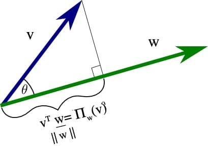
Projections

In linear algebra, the scalar projection of a vector v ∈ ℝ^d onto vector w ∈ ℝ^d is the scalar projection \(\Pi_w (v) = v^T \frac{w}{‖w‖}\)

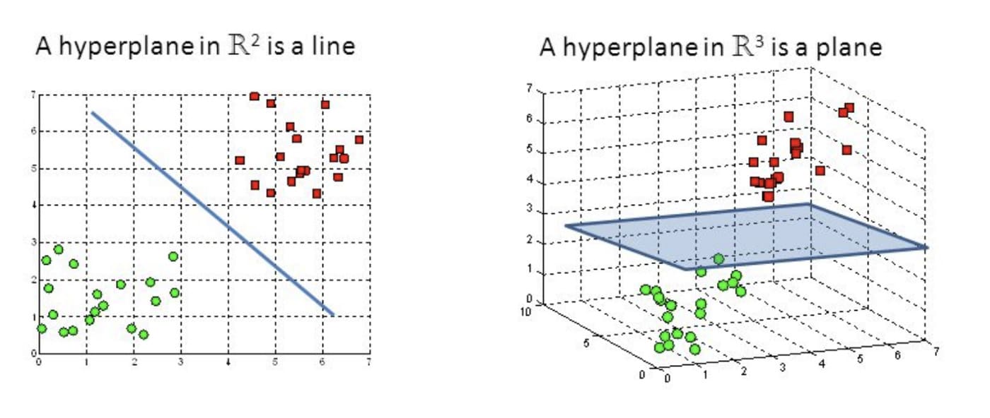
Hyperplanes and Distances

Hyperplane can be considered as decision boundaries, that classify data points into classes in multi-dimentional space. Data point will be located on the either side of a hyperplane. A hyperplane is a generalization of a plane. In two dimension, it’s a line. In three dimention, it’s a plane. In more dimentions it will be a hyperplane.

In the line, we usually define line as y=ax+b . it will the same as on the hyperplane, we get \(w^T x + b\)

An (affine) linear function is a function f : ℝ^d → ℝ of the form \(f(x) = w^T x + b\), where w ∈ ℝ^d (w ≠ 0) and b ∈ ℝ.

A hyperplane is a subset H ⊂ ℝ^d defined as \(H := \{ x \in ℝ^d : f(x) = 0 \}\)

The preposition or properties of hyperplanes. Let H be a hyperplane defined by the affine-linear function \(f(x) = w^T x + b\)

• the vector w is orthogonal to H, meaning that: for all x₁, x₂ ∈ H. it holds \(w^T (x_1 - x_2) = 0\)
• the signed distance of a point x to H is given by \(d(x,H) = \frac{1}{ \lVert w \rVert }(w^Tx+b)\)

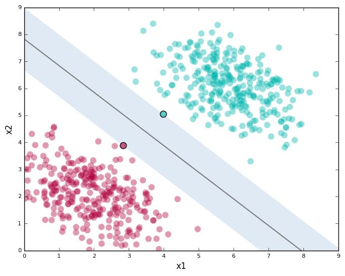
Finding the best Hyperplane

By looking at the data points and the result hyperplane, we can see the margin between the data with the hyperplane. This mean that the optimal hyperplane will be the one with the biggest margin, because the large margin will give a small deviation in the data points, and will not effect with the outcome of the model.

Linear Classifiers

A classifier of the form \(f(x) = w^T x + b\) is called linear classifier.

Adventages

• They easy to understand
• It works really well on clear margin seperation
• It is still effective on the big data, and also effective in cases where the number of dimensions is greater than the number of samples.
• It is fast

Disadventages

• Suboptimal performance if true decision boundary is non-linear. it occure for very complex problems such as recognition problem and many others.

Nearest Centroid Classifier

NCC is the linear classifier that classifies model that assigns to observations the label of the class of training samples whose the mean or (centroid) is closest to the observation.

The training data is compute as plus and minus centroid. by computing centroid for each using \(c_{-} = \frac{1}{ \vert I_{-} \vert } \sum_{i \in I_{-}} x_i\) for negative and \(c_{+} = \frac{1}{ \vert I_{+} \vert } \sum_{i \in I_{+}} x_i\) for positive.

The prediction is given new x predict using \(arg min_{y \in \{ - , +\}} ‖ x - c_y ‖\)

Proof if the NCC is linear classifier \(f(x) = w^T x + b\) with \(w:= 2(c_+ - c_-)\) and \(b := ‖c_-‖^2 - ‖c_+‖^2\)

The decision boundary is \(H = \{ x \in ℝ^d : \| x - c_- \| = \| x - c_+ \| \}\)

\[\| x - c_- \|^2 = \| x - c_+ \|^2\] \[\| x \|^2 - 2c_-^T x + \| c_- \|^2 = \| x \|^2 - 2c_+^T x + \| c_+ \|^2\] \[2(c_+ - c_-)^T x + ( \| c_- \|^2 - \| c_+ \|^2 )\]

\(w:= 2(c_+ - c_-)\) and \(b := ‖c_-‖^2 - ‖c_+‖^2\)

\[w^T x + b = 0\]

Thus it is proved that the NCC is a linear classifier.

Linear Support Vector Machines

The properties of Linear SVMs is fast. It can be trained in O(n d) . it also can be trained in a distributed manner (map-reduce). The second is the Linear SVMs is simple. it will easy on the geometrical interpretation. the third is accurate, in circa 50% of the data out there.

State of the art in many application area, for example in gene finding which is find in the DNA the positions that impact virtually all important inherited properties of human e.g. intelligence, height, visual appearence, etc.

There are two types of Linear SVM: Hard-margin linear SVMs and Soft-margin linear SVMs.

Hard-Margin Linear SVM

The core idea of the Hard-margin Linear SVM is to make the hyperplane separates the data with the largest margin. So the goal is maximize the margin such that all data points lie outside of the margin.

How we can matematically do this, so we can tell the computer what the computer should do. We can start with denote the margin by γ (gamma), then find the hyperplane parameters w and b that maximize the margin γ. But, also make sure that all positive data points lie on one side and all negative points on the other side.

• a point \(x_i\) with \(y_i = +1\) lies on correct side of margin if \(d(x_i,H) \geq +\gamma\)
• a point \(x_i\) with \(y_i = -1\) lies on correct side of margin if \(d(x_i,H) \leq -\gamma\)

Hence, we require for all points \(x_i\), is represented as \(y_i \cdot d(x_i,H) \geq \gamma\). So by using this equation, find the hyperplane H with maximal margin γ such that (s.t.) for all training points \(x_i\) it holds: \(y_i \cdot d(x_i,H) \geq \gamma\)

Preliminary formulation of SVM :

We recall the hyperplane H is parametrized by w and b through: \(H = \{ x : w^T x + b = 0 \}\). and the previous proposition that \(d(x,H) = \frac{1}{ \lVert w \rVert }(w^Tx+b)\)

\(\underset{\gamma, b \in ℝ, w \in ℝ^d}{\max} \ \ \ \gamma\) such that

\[y_i \ ( w^T x + b ) \geq \| w \| \ \gamma , \ \ \forall i = 1,...,n\]

Limitations of Hard-Margin SVMs

Any three points in the plane \(ℝ^2\) (not lying on a line) can be “shattered” or separated by line (linear classifier). But there are configurations of four points which no hyperplane can shatter.

Any n+1 points in ℝⁿ (not lying in a hyperplane) can be “shattered” by a hyperplane. But there are configurations of n+2 points which no hyperplane can shatter.

Another problem is that of outliers potentially corruption the SVM.

Soft-Margin Linear SVM

The core ide of the soft margin is introduce for each input \(x_i\) a slack varible \(\xi \geq 0\) that allows for some (slight violations of the margin separation):

Linear Soft-Margin SVM

\[\underset{\gamma, b \in ℝ, w \in ℝ^d, \xi_i,...\xi_n \geq 0 }{\max} \ \ \ \gamma - \color{red}{ C \sum_{i=1}^{n} \xi_i }\]

such that

\[y_i \ ( w^T x + b ) \geq \| w \| \ \gamma - \color{red}{ \xi_i }, \ \ \forall i = 1,...,n\]

• Minimizes \(C \sum_{i=1}^{n} \xi_i\), to allow for “slight” violations of the margin.

• \(C \sum_{i=1}^{n} \xi_i\) is the total amount of violations of the training points lying inside the margin (measured in distances to the margin)

• C > 0 is a trade-off parameter (to be set in advance): the higher C, the more we penalize violations. Higher C is harder SVM, and lower C is softer SVM. When C is small, classification mistakes are given less importance and focus is more on maximizing the margin. When C is large, the focus is more on avoiding misclassification at the expense of keeping the margin small.

Why the name ‘Support Vector Machine’?

Since the margin is calculated by taking into account only spesific data points, support vectors are data points that closer to or inside the tube of the hyperplaneand influence with the orientation and the position of the hyperplane.

Assume we denote the optimal arguments from the previous equation by \(\gamma^* \ and \ w^*\).

The definition, All vector \(x_i\) with \(y_i \cdot d(x_i,H(\gamma^*, b^*)) \leq \gamma^*\) (i.e., lying inside the tube) are called support vectors. The SVM depends only on the support vectors: all other points can be removed from the training data (no impact on classifier)

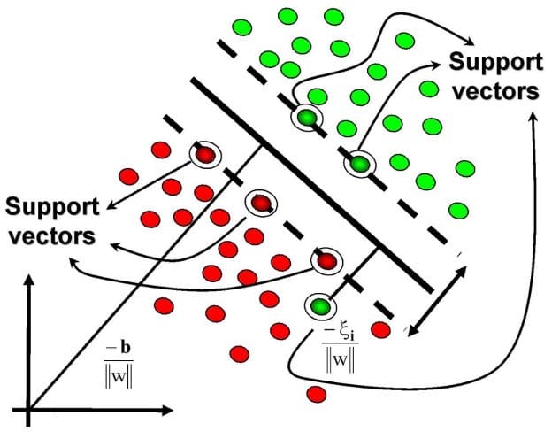
The support vectors are imaginary or real data points that are considered landmark points to determine the shape and orientation of the margin. The objective of the SVM is to find the optimal separating hyperplane that maximizes the margin of the training data.

Conclusion

• Linear Support Vector Machines (SVMs) motivated grometrically by the image on the title.
• Mathematical formalization of the image is

\[\underset{\gamma, b \in ℝ, w \in ℝ^d}{\max} \ \ \ \gamma\]

such that

\[y_i \ ( w^T x + b ) \geq \| w \| \ \gamma , \ \ \forall i = 1,...,n\]

• This idea for Soft Margin SVM is based on a simple premise: allow SVM to make a certain number of mistakes and keep margin as wide as possible so that other points can still be classified correctly. This can be done simply by modifying the objective of SVM.